A Machine Learning Approach to Constructing an Inflation-Themed Equity Portfolio

In this Street View, we analyze the historical relationship of equity sectors and style factors with inflation. We then present a machine learning model that can be used to construct a thematic equity portfolio that should outperform in high inflation periods and underperform in low inflation periods.

One of our most recent Street Views covered the topic of inflation, an important driver of markets today, and how one could approach inflation forecasting like a data scientist by analyzing it from as many perspectives as possible. Once one has a forward-looking view on inflation, one can use that information to position their portfolios accordingly. Common ways to express a view on inflation are through Treasury Inflation-Protected Securities (TIPS) or gold, as these are two inflation-sensitive assets (one mechanically and one theoretically). Another, perhaps less common way, could be to express a view using the largest component of most multi-asset portfolios: stocks.

Equity Behavior in Different Inflation Environments

In this section, we’ll explore how the overall equity market has performed in different inflation environments and analyze the results cut across sectors and styles.

As an initial matter, one should first understand where inflation stands today as compared to its history. Exhibit 1 plots the historical year-over-year values for the Consumer Price Index (CPI) and Core CPI, which excludes food and energy. We define “High Inflation” as periods where inflation is greater than 3%, “Medium Inflation” as periods where inflation is between 1 and 3%, and “Low Inflation” as periods where inflation is less than 1%. These thresholds roughly correspond to the Federal Reserve’s perceived inflation tolerance. However, as we mentioned in our prior Street View, there are many ways to measure inflation, and these are just two. The main takeaway here is that while inflation (at least as measured by CPI¹) is “high” today, it’s certainly not yet as high as the levels experienced in the 1970s and 1980s.

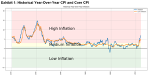
Exhibit 2 plots the monthly returns of the U.S. equity market (y-axis) versus year-over-year U.S. CPI in the same month as the equity market return (x-axis). The red line is the best fit line, and it exhibits a negative slope.²

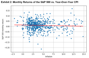
The relationship between these two variables is complicated.³ While there are many factors that may influence the relationship between inflation and equity market returns, one might expect that high levels of inflation are negative for overall equity markets. If the U.S. Federal Reserve raises interest rates in response to higher inflation, the higher borrowing costs might hurt companies because the present value of the discounted cash flows falls when the discount rate is higher. However, because equities can represent claims on tangible assets, higher inflation could benefit them in the same way inflation benefits assets like real estate. Another case where equity markets may benefit from higher inflation is if that high inflation is partnered with positive economic growth. So, while it may be a general expectation that equity markets underperform when inflation is high, it’s not a certain conclusion, and it really depends on the scenario and drivers of inflation.

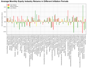
Next, we’ll explore how various breakdowns of the equity market typically behave in different inflation environments. First, let’s look at equity sectors (see the Appendix for the average monthly stock returns by industry). In Exhibit 3, we calculate each sector’s average monthly return in High, Medium, and Low Inflation periods, as defined above.

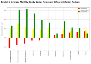
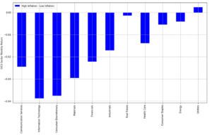
Sources: Bloomberg and Barra. Period: August 1997 – December 2021, using monthly data.

Returns were lower in the High Inflation periods for almost all equity sectors. The return difference between High and Low Inflation periods is most stark for Information Technology, Consumer Discretionary, and Materials. On the other hand, there is almost no difference for the Utilities sector, perhaps because utilities are critical for survival so demand is less elastic.⁴

Next, we take a look at equity style factors. We construct quartile portfolios that are positioned long (short) the top (bottom) 25% of stocks, according to each stock’s style factor loading. Then, we compare the style portfolios’ average monthly returns in High, Medium, and Low Inflation periods.

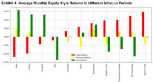
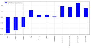
High Inflation has resulted in lower returns for the Beta, Growth, and Prospect styles.⁵ On the other hand, Earnings Quality, Dividend Yield, Management Quality, and Earnings Yield outperformed in the High Inflation environment. This generally matches fundamental intuition: when using a discounted cash flow model to evaluate the intrinsic value of a company, a growth stock will typically have a relatively greater portion of their intrinsic value coming from the more distant future, while value-oriented stocks (i.e., those with high earnings yields, dividend yields, etc.) tend to have a relatively greater portion of their intrinsic value coming in the nearer term. Since the discount factor, which is used to discount future cash flows to the present, increases as inflation increases, growth stock cash flows will be more heavily discounted when calculating present value. The opposite is true for value stocks, where cash flows are less heavily discounted.

Using Machine Learning to Construct an Inflation-Themed Equity Portfolio

Now that we have an understanding of equity behavior in different inflation environments, we can build an equity-based thematic portfolio that is responsive to inflation. One way to construct that portfolio might be to simply overweight the sectors that perform well in High Inflation environments and underweight those that don’t. You could also use a factor-based optimizer that sets constraints around the active exposures to style factors, again making sure to have more weight towards styles that outperform in High Inflation environments and less weight towards those that underperform.

An alternative approach would be applying machine learning or some other form of statistical modeling. In this Street View, we’ll provide one example of that alternative, using a supervised machine learning model called LightGBM (or Light Gradient Boosting Machine).⁶ We selected this particular model for its high efficiency (fast training speed and low memory usage), support of distributed learning, and ability to easily customize the loss function.⁷ However, this is just an example use case – our intent is to simply show a real-life application of using machine learning to help construct portfolios that can be sensitive to market themes like inflation. The model will help us construct a beta-neutral portfolio of individual stocks that is specifically designed to outperform in High Inflation periods and underperform in Low Inflation periods.

Model Set Up

The primary input to the model is a large data set that includes:

• Historical High and Low Inflation period data (using CPI)⁸
• The stock returns in those High and Low inflation periods⁹
• Sector and style factor loadings for each stock
• Fundamental data, like employee size and profit margins for each stock
• Forecasted data, like analyst predictions of future earnings for each stock

The data is from January 2005 to September 2021, and we use a walk-forward approach, making sure that the model is trained using historical data only (i.e., the model does not have access to any future information). Admittedly, the data history is not very extensive (it starts in 2005 and therefore excludes High Inflation periods like the 1970s and 1980s), so we make several adjustments to the model to boost training and reduce overfitting.¹⁰

The output of the model is a list of features, or variables, and their relative importance when fitting a model that best predicts stock returns in High and Low Inflation periods. One can think of the model’s output like that of an equation where a stock’s predicted return is a function of its sensitivities, or betas, to certain variables (like those listed above: sector loadings, profit margins, analyst earnings predictions, etc.).

In a standard Ordinary Least Squares regression, the loss function seeks to minimize the model’s “errors” – that is to minimize the sum of the differences between model-predicted values and actual values for all data provided to the model. The model cares about all points in the data set equally. The loss function in the LightGBM model we propose here is a bit different. In the specification of the LightGBM model’s loss function, we encourage the model to put more weight on correctly predicting the returns in the tails of the data set – that is the stocks that perform best (worst) when inflation is high (low).

Model Results

Now for the model’s results: we find that there are a few features, or variables, that the model reveals to be relatively important.

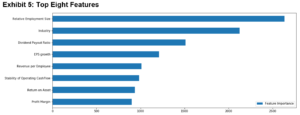
We’ll discuss several of these top features:

• Relative employment size: this can be viewed as a proxy of the stock’s sensitivity to wage inflation
• Industry: this is expected since, as we observed in Exhibit 3, there are some sectors (and industries) that are more sensitive to inflation than others
• Dividend payout ratio: as expected, value stocks with nearer-term cash flows are less impacted by rising inflation
• Profit margin: perhaps companies with high profit margins have a better chance of surviving in High Inflation periods

Model Application

We use the fitted model to build an equity portfolio, which we’ll call the “Model Equity Portfolio,” that should be sensitive to inflation. To form the Model Equity Portfolio, we hold 10% of the stocks with the highest predicted returns using the fitted model. Our starting universe of stocks is ~800 of the most liquid large cap stocks in the U.S., so this leaves us with a portfolio of ~80 stocks, which we believe to be fairly standard for a thematic equity portfolio (the portfolio will have some diversification to reduce single stock risk, while at the same time still strongly representing the inflation theme we want to express).

To test the model’s success, we can evaluate the Model Equity Portfolio’s active returns (i.e., returns in excess of the S&P 500 Index) in High and Low Inflation periods. Again, we are taking a walk-forward approach, using only historical data (i.e., no future information) to construct the portfolio at each point in time. Our data set starts in 2005 and ends in 2021. As a reminder, the Model Equity Portfolio is designed to perform well in High Inflation periods and poorly in Low Inflation periods. It is not an alpha-seeking portfolio, so we should not necessarily expect it to have a positive return over the long-term. Keep in mind that this model is not predicting inflation itself. Rather, it simply seeks to construct a portfolio of stocks that will perform well when inflation is high.

We indeed see from the leftmost red bar in Exhibit 6 that the Model Equity Portfolio performed well during High Inflation months on average. If we attribute this positive average return in High Inflation periods to the portfolio’s active sector and style exposures, we find that most of the positive return is coming from residual (perhaps because the Barra model we use for attribution doesn’t have an inflation factor) and some from the portfolio’s active style exposures. Interestingly, the active sector exposures detracted from the portfolio’s average outperformance in High Inflation periods.

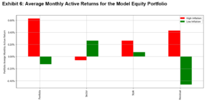
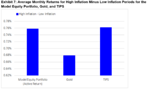
In Exhibit 6, we find that the Model Equity Portfolio’s average active return in High Inflation periods minus Low Inflation periods is approximately 0.8% (we take the leftmost red bar and subtract the leftmost green bar). In Exhibit 7, we see how that outperformance in High Inflation periods over Low Inflation periods compares to other inflation-hedging instruments: gold and TIPS. The Model Equity Portfolio was on par with that of TIPS, and it outperformed gold.

Another way to test the model’s success is to analyze the Model Equity Portfolio’s average sector and style factor exposures to understand the extent to which they align with the analysis we presented earlier in this Street View (in Exhibits 3 and 4 when we showed the average sector and style returns in different inflation periods). That is, the portfolio may exhibit positive average exposures to sectors and styles that perform well in High Inflation environments and negative average exposures to those that don’t.

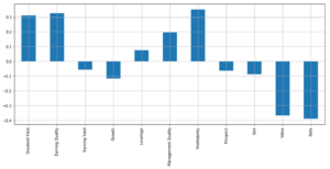
In Exhibit 8, we find that the Model Equity Portfolio had positive active sector exposures to Consumer Staples, Healthcare, and Utilities and negative active exposures to Information Technology, Financials, and Energy. In terms of styles, the Model Equity Portfolio was positively tilted toward stocks with high dividend yields, profitability, and earnings quality and negatively tilted toward high-beta, value, and growth stocks.

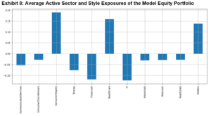
Sources: Bloomberg, CIQ, Compustat, Worldscope, IBES, and Barra. Period: January 2010 – December 2021, using monthly data. The portfolio was trained with monthly data starting from January 2005.Some of these results line up with the analysis earlier, such as the positive Utilities and Earnings Quality exposures, and the negative Information Technology and Growth exposures. As we mentioned in a prior Street View, one of the advantages of the machine learning approach is that it is entirely data-driven—that is, the model outputs features and their relative importance when fitting a model that best predicts stock returns in High and Low Inflation periods, but the features won’t necessarily map exactly to what we or others could have specified ex-ante. This is both bad and good. Bad in the sense that it might be hard for us to put intuition behind the resulting Model Equity Portfolio’s exposures, and good in the sense that it will hopefully tell us something that we wouldn’t have known without employing a technique like machine learning.

Conclusion

Market participants are becoming increasingly concerned about rising inflation and its effect on their portfolios. Equity risk is the primary driver of most institutional multi-asset class portfolios, so how should investors think about allocating within their equity portfolio to withstand potentially higher inflation?

This analysis looked at inflationary periods historically and examined how different components of the equity universe – sectors and styles – performed in those periods. While positive inflation tends to result in lower returns for the equity market overall, there are certainly pockets of the equity market that can do well in these environments. We then presented a machine learning-based approach to construct an equity portfolio that is specifically designed to outperform in High Inflation periods.

All that said, this specific model was meant to be a practical, yet illustrative example. There are many modifications one can make to this analysis, including:

• The measure of inflation used (we used CPI, but there are so many other ways to look at inflation as we discussed in a prior Street View)
• The region in which inflation is measured (we analyzed the U.S., but one could look ex-U.S. where there may be significantly more recent High Inflation data)
• The definitions for High and Low inflation (we selected 3% and 1% cut-offs, respectively)
• The data provided to the model (we used a combination of fundamental, forecasted, and sector and style loadings data)
• The selection of the model itself (we used a LightGBM)

Perhaps the most important takeaway from this analysis is the ability to use techniques like machine learning to practically assist with portfolio construction.

Appendix